Feature selection part 2
A critique to feature importance
In part 1, I showed some of the dangers of using univariate selection methods. In part 2 I want to focus on the pitfalls of feature importance in random forests and gradient boosting methods.
I’ll write about it in the feature selection chapter as feature importances can be used to select features, as in Sklearn SelectFromModel.
In order to select features using feature importances, one can:
- Train a model that has allows to compute feature importances.
- Retrain the model with only the most important features.
In my experience, when retraining with only the most important features, the model usually degrades a little.
The main issue regarding selecting features using feature importance is that, if a feature is highly correlated with others, its importance will be lower than if it isn’t correlated with any features. For this reason I advise to check that your features are not very correlated if you want to assess them using feature importance.
Experiment set-up
In order to show the issues of selecting features using feature
importance, we’ll use a rather ill-defined example. In this example,
x1, x2, x3 and x4 are independent variables and the dependent
variable is
y ~ x1 + (x2 + x3 + x4) * 0.5 + noise
When training a random forest, x1 should appear as the most important
variable. If the feature selection method had to keep only one feature,
x1 should be the one to select.
To see an example where feature importance might mislead you, we’ve
created some brothers to x1. They are variables that are very
correlated to x1 and will be used to model y as well. These brothers
are what cause the importance of x1 to be diminished.
library("dplyr")
library("randomForest")
library("glmnet")

set.seed(42)

len <- 5000

x1 <- rnorm(len)
x2 <- rnorm(len)
x3 <- rnorm(len)
x4 <- rnorm(len)

# The outcome is created without the brothers
y <- x1 + 0.5 * x2 + 0.5 * x3 + 0.5 * x4 + rnorm(len)

# x1i are x1's "brothers": variables that are mainly x1 but with some noise
x11 <- 0.95 * x1 + 0.05 * rnorm(len)
x12 <- 0.95 * x1 + 0.05 * rnorm(len)
x13 <- 0.95 * x1 + 0.05 * rnorm(len)
x14 <- 0.95 * x1 + 0.05 * rnorm(len)
x15 <- 0.95 * x1 + 0.05 * rnorm(len)
x16 <- 0.95 * x1 + 0.05 * rnorm(len)
x17 <- 0.95 * x1 + 0.05 * rnorm(len)
x18 <- 0.95 * x1 + 0.05 * rnorm(len)
Then we create the feature matrix, with x1 to x4, as well as x1’s
brothers.
model_tbl <- tibble(
  y = y,
  x1 = x1,
  x2 = x2,
  x3 = x3,
  x4 = x4,
  x11 = x11,
  x12 = x12,
  x13 = x13,
  x14 = x14,
  x15 = x15,
  x16 = x16,
  x17 = x17,
  x18 = x18
)

X <- as.matrix(select(model_tbl, -y))
Random forest importance
A random forest model is trained (when training this model, it automatically computes feature importance).
rf <- randomForest(X, y, importance = T)
And we show the importance of the features:
varImpPlot(rf, type = 1)
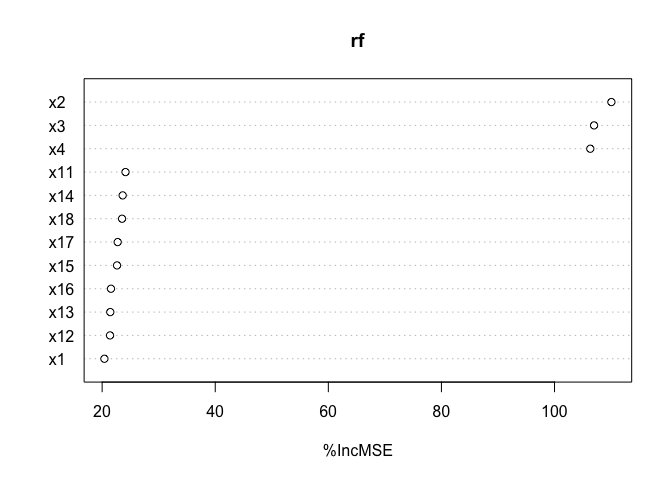
This shows the shortcomings of feature importance: x1 doesn’t appear
as the most important feature. If we were to select three variables, we
would select x2, x3 and x4, and this would of course degrade the
model performance.
Thinking about it, it makes sense. In this random forest, to model the
x1 contribution, some splits are done with x1, some with her
brothers. For this reason, if x1 gets broken, the impact is not as big
as if x2 breaks.
Lasso selection
On the other hand, lasso kind of makes it (recall that cv.glmnet
default is lasso):
# Train lasso
lasso <- cv.glmnet(X, y)

# Kind of makes it
coef(lasso, s = "lambda.min")
## 13 x 1 sparse Matrix of class "dgCMatrix"
##                      1
## (Intercept) 0.01334871
## x1          0.90829549
## x2          0.49467345
## x3          0.49902516
## x4          0.48559226
## x11         0.01570838
## x12         .
## x13         .
## x14         .
## x15         .
## x16         0.02241166
## x17         0.06331782
## x18         .
It selects some of the x1 brothers, but with really small
coefficients. If we regularize a bit more, they’ll probably vanish.
In fact, the next figure shows that the last feature to be vanished is
x1, which didn’t happen in the random forest:
# x1 is the last one to go
plotmo::plot_glmnet(lasso$glmnet.fit)
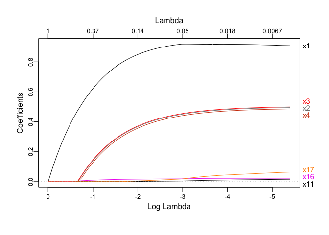
Of course Lasso selects the variables better in this case, as the model is generated linearly. A case where feature importance might shine more than the Lasso is when the dependent variable is a non-linear function of the features.
To sum up, be careful with feature importance when having highly correlated features.