Non-normality
It's not that bad
I’m still reading the great Statistical Rethinking book by Richard McElreath, and I’m learning plenty of things. One thing it quickly mentions is that you shouldn’t worry about having non-normal data when using a linear regression. Linear regression can be defined as
y ∼ N(a0 + a1x1 + … + anxn, σ2)
This doesn’t imply that y has to be normally distributed in our data. It only means that y needs to be normally distributed conditional to x. Let’s do an experiment to show this.
We’ll generate x using a beta distribution, thus generating a very skewed distribution for x. We’ll generate y by adding some small noise to x.
# Libraries

library(dplyr)
library(ggplot2)

theme_set(theme_minimal())
n <- 100000

# Create x, noise and y
x <- rbeta(n, 2, 5)
noise_y <- rnorm(n, 0, 0.01)
y <- x + noise_y

# Prepare data and plot y
df <- data.frame(x = x, y = y)

ggplot(df) +
  geom_density(aes(x = y))
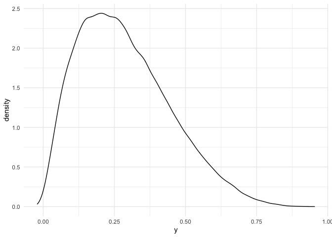
As we can see, y is pretty skewed. A naive statistician might say that, being the data not normal, we should not fit a plain linear model, as this assumes normality of data. Keep in mind that the linear model assumes normality of the data conditioned on the predictors, so this might be a situation in which a linear model still makes sense.
# Fit linear regression
model <- lm(y ~ x, data = df)

# Compute residuals
predictions <- as.vector(predict(model, df))
df$error <- y - predictions

# Show residuals
ggplot(df) +
  geom_density(aes(x = error))
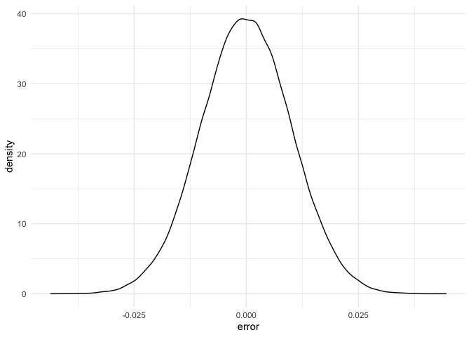
As we can see, the distribution for the error is not skewed anymore, it looks like a normal. Let’s check it with a qqplot:
ggplot(df) +
  stat_qq(aes(sample = error)) +
  stat_qq_line(aes(sample = error))
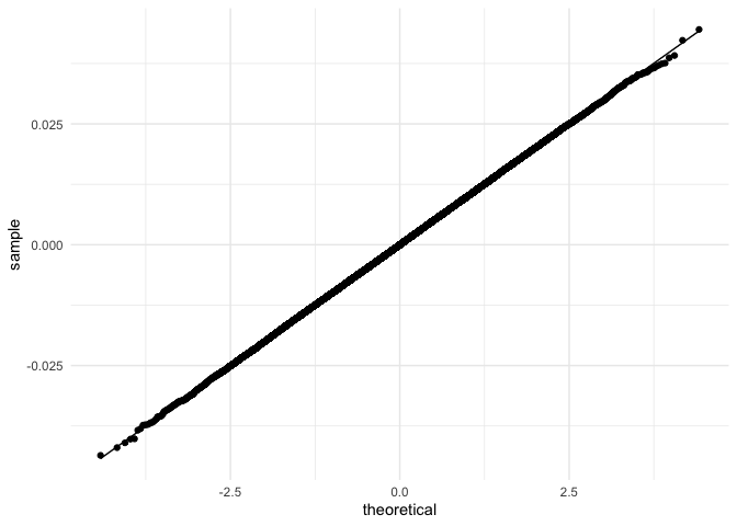
Indeed, the residuals follow a normal distribution.
To sum up, having a non-normal target doesn’t mean that the linear model is not suitable. If the residuals from the linear model follow a normal distribution, then the linear model is an appropiate one.